← Introduction → Continuous Contraction Semigroups
What should you be acquainted with? Measure Theory and some basics in Functional Analysis.

Examples

Discrete Dynamical Systems

In the sequel (Ω,F,μ) will always denote a σ-finite measure space. All spaces S are more or less assumed to be Polish, i.e. there is some metric d on S such that (S,d) is a complete and separable metric space. This ensures in particular that SN is Polish and the Borel σ-algebra B(SN) on SN coincides with the product σ-algebra, e.g. F:ΩSN is measurable iff all components PrnF are measurable. Morover any finite Borel measure μ on S is regular, i.e. for all Borel sets A and all ϵ>0 there is a compact set K and an open set U, such that KAU and μ(UK)<ϵ. It follows that e.g. bounded Lipschitz functions are dense in Lp(μ) for all 1p<:
Put f(x)=d(x,Uc)d(x,Uc)+d(x,K), then f is Lipschitz, f|K=1, f|Uc=0 and for all p>0: |fIA|pdμ<ϵ. Solution by T. Speckhofer
If S=M is a (smooth) manifold (i.e. for convenience, a connected Polish space locally homeomorphic to a euclidean space with a differentiable structure). If you don't care about manifolds in general, open subsets of euclidean spaces suffice - though we assume that all manifolds don't have a boundary! The space Cc(M) of smooth functions with compact support is dense in Lp(μ) for all 1p< and all Radon measures μ on M, i.e. μ is Borel and all compact subsets of M have finite measure.
A measurable mapping θ:SS is called measure preserving if for all AF: μ(θA)=μ(A) i.e. the image measure μθ of μ under θ equals μ.
Thus θ is measure preserving, if μ is invariant under the mapping θ. We will also say that μ is stationary under θ and call (S,F,μ,θ) a dynamical system. By the transformation theorem of measure theory θ:SS is measure preserving if and only if for all fL1(μ): fθdμ=fdμ . Suppose θ is measure preserving, then for all fLp(μ) and all nN0 we define Pnf(x):=f(θn(x)) where θ0(x):=x. This is a simple example of what is known as a semigroup Pn on Lp(μ); since θ is measure preserving, we have: Pnfp=fp, in particular Pn is a contraction semigroup.
Put S=T:=R/2πZS1 and let λ(dx)=dx/2π be the normalized Haar measure on T. Then for all θR the mapping Θ:S1S1, zze2πiθ (or Θ:TT, xx+2πθ) is measure preserving.
Put S=[0,1) and θ(x)=2x(mod1). Then the Lebesgue measure is invariant under θ.
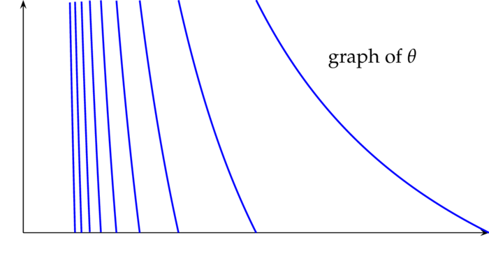
θ:(0,1)(0,1) has an invariant measure with density ρ iff (cf. exam): x(0,1):y:θ(y)=xρ(y)|θ(y)|=ρ(x) .
Put θ:RR, θ(x)=x1/x. Then the Lebesgue measure is θ-invariant. Cf. example.
Suppose θ:R+R+ is an increasing bijection. Then μθ(0,θ(x))=μ(0,x).
Suppose θ:SS has a fixed point xS, i.e. θ(x)=x. Then δx is θ-invariant.
Put S=[0,1) and θ(x)=ax(mod1) for a1=1/a, a>0. Then Lebesgue measure is not invariant under θ. Find a measure μ on S invariant under θ. Hint: Assume μ has constant density m1 on (0,1/a) and constant density m2 on (1/a,1). Suggested solution
Show that the map θ:(0,1)(0,1) θ(x):={x1xif x(0,1/2]1xxif x(1/2,1) has an invariant measure with density 1/x.
Suppose μ is a Borel probability measure on the Polish space S and let P be the product measure on Ω:=SN. The so called shift operator Θ:ΩΩ defined by Prn(Θ(ω))=ωn+1 is obviously measurable (with respect to the product σ-algebra) and P is invariant under Θ. Θ is also known as the Bernoulli shift and the dynamical system a Bernoulli scheme (cf. exam).
Since the Borel σ-algebra of Ω is generated by the projections Prn, nN, we only have to show that for all AB(S) and all nN: P(Θ[PrnA])=P([PrnA]). Now by definition P([PrnA])=μ(A) and since PrnΘ=Prn+1 we conclude that P(Θ[PrnA])=P(PrnΘA)=P(Prn+1A)=μ(A) . Remark: In probability the projections Prn are independent and identically distributed S-valued random variables, a so called i.i.d. sequence in S with distribution μ.
On S=[0,1] define θ:SS by θ(x)={2xif x<1/22(1x)x1/2 Then the Lebesgue measure is invariant under θ. Similarly θ(x)=2x[2x] on [0,1] or on [0,1)=R/Z: θ(x)=2xmod(1).
On the set S=[0,1]2 define θ(x,y)={(2x,y/2)if x<1/2(22x,1y/2)x1/2 Then the Lebesgue measure is invariant under θ. The transformation θ is known as the folded baker transformation. Suggested solution. Solution by T. Speckhofer. The unfolded baker transformation θ:SS is given by θ(x,y)=(2x[2x],(y+[2x])/2), cf. e.g. wikipedia. Both the folded and the unfolded map are invertible!

The Gauß map

On the set S=[0,1) define the Gauss map θ(x)=1/x[1/x]. Now let μ be the probability measure on S with density (log2)1(1+x)1, then μ is θ-invariant.
gauss map
For 0<t<1 we have μθ((0,t])=μ(0<θt). x[0<θt], iff 1/x[1/x]+t, i.e. 1/x[n,n+t] and this holds if and only if x[1/(n+t),1/n]. log2μθ((0,t])=n=11/(n+t)1/n11+xdx=n=1log1+1/n1+1/(n+t)=n=1(log1+n1+n+tlognn+t)=log11+t=log2μ((0,t]) .
Let θ be the Gauss map. For real numbers x1,,xk1 put x1:=1x1andx1,,xk+1=1x1+x2,,xk+1 . In particular: x1,x2=1x1+1x2,x1,x2,x3=1x1+1x2+1x3, Provided θk(x)0 define for x(0,1): a1,a2,:(0,1)N by a1(x):=[1/x],ak+1(x):=[1/θk(x)] . The sequence a1(x),a2(x), is called the continued fraction of x. Verify the following statements: (suggeted solution)
  1. For all x[0,1) and all kN such that x,θ(x),,θk1(x)0: x=a1(x),,ak(x)+θk(x)andθ(x)=a2(x),,ak(x)+θk(x) .
  2. For n1,,nkN and t(0,1): θ(n1,,nk+t)=n2,,nk+t .
  3. Put I=[0,1)Q. For all kN we have θk(I)I. Hence the functions ak:IN are defined for all kN.
  4. For all x[0,1)Q there is some kN such that θk(x)=0. Conversely, if θk(x)=0, then x must be rational.
For n1,n2,N we put In1:=(n1+1,n1),In1,n2:=(n1,n2,n1,n2+1),In1,n2,n3:=(n1,n2,n3+1,n1,n2,n3,etc. Then the following holds (suggested solution):
  1. θ is a homeomorphism from In1,,nk onto In2,,nk.
  2. In1,,nk,nk+1In1,,nk.
  3. For all jk: aj|In1,,nk=nj.
  4. The open interval In1,,nk has length at most 2k. Thus if aj(x)=aj(y)=nj for all jk, then |xy|2k.
The mapping a:INN, x(an(x)) is a homeomorphism with inverse (n1,,nk,)limkn1,,nk.

An example on the real line

Suppose αR, a1<a2<<an, a0=, an+1= and c1,,cn>0. Define θ:RR by θ(x):={x+αj=1ncj(xaj)1if x{a0,,an+1}if x{a0,,an+1}
  1. For all tR the equation θ(x)=t has exactly n+1 real solutions xj(t) and aj<xj(t)<aj+1.
  2. j=0nxj(t)=1 and for all fL1(R): fθdλ=fdλ .
1. θ|(aj,aj1) is continuous, θ>1 and limxajθ(x)=,limxaj+1θ(x)= . Moreover limx±θ(x)=±.
2. Fix tR and put q(x):=(xx0)(xxn), p(x):=(xa1)(xan)=xnxn1aj+ and pj(x)=p(x)/(xaj). Then q(x)=(θ(x)t)p(x)=(x+αt)p(x)j=1ncjpj(x)=x(xnxn1aj)+(αt)xn+r(x), where r is some polynomial of degree n1 at most. Comparing the coefficients of xn we find: j=0nxj=j=1naj+αt . Therefore θ:(aj,aj+1)R is a diffeomorphism with inverse xj and by the transformation theorem of measure theory: fθdλ=j=0n+1ajaj+1f(θ(x))dx=j=0n+1f(t)xj(t)dt=fdλ .
Lebesgue measure on R+ is invariant under θ(x)=|x1/x|.
Verify that Rex21/x2dx=πe2 .
For t>0 let μt be the measure on R+ with density xtexp(t2/4x)4πx3 . Show that the Laplace transform ωt(y):=0exyμt(dx) is given by ωt(y)=ety. 2. Conclude that μsμt=μs+t. The measures μt are called 1/2-stable probability measures on R+ (1/2 refers to the square root of y in ωt). Suggested solution.

Homomorphic and isomorphic systems

A dynamical systems (S~,F~,μ~,θ~) is said to be homomorphic to (S,F,μ,θ), if there is a measurable mapping F:(S,F)(S~,F~) such that μ~=μF and θ~F=Fθ. If in addition (S,F,μ,θ) is also homomorphic to (S~,F~,μ~,θ~), then (S,F,μ,θ) and (S~,F~,μ~,θ~) are said to be isomorphic.
If μ is θ-invariant, then μF is θ~-invariant, because for all BF~ we have by definition: μF(θ~1(B))=μ(F1(θ~1(B)))=μ((θ~F)1(B))=μ((Fθ)1(B))=μ(θ1(F1(B)))=μ(F1(B))=μF(B) . Suppose R is an equivalence relation on a Polish space S such that S/R is again Polish. Let π:SS/R be the quotient map. If a continuous map θ:SS is constant on all sets R(x), then there is a continuous map θ^:S/RS/R such that θ^π=πθ. Finally, if μ is a θ-invariant probability measure on S, then its image measure μπ is θ^-invariant.
For S:=(0,1) and θ(x)=4x(1x) let μ be the probability measure with density f(x)=π1(x(1x))1/2. Then μ, δ0 and δ3/4 are θ-invariant. Moreover, put F(x)=(sin(πx)/2)2, then (suggested solution) F1θF(x)={2xif x<1/22(1x)if x1/2
Let S=R+, μ(dx)=exdx and θ(x)=log|12ex|. Then μ is θ-invariant. Suggested solution.

Recurrence

Suppose θ is a measure preserving map on the probability space (Ω,F,P). Then for all AF: P(Alim supn[θnA])=P(A) .
Proof: Let B be the set of all ωA, such that for all k1: θk(ω)A, i.e. B:=Ak1[θkAc]=Ak1θk(Ac) . Then for all n1: Bθn(B)=, for θn(B)θn(A) and Bθn(Ac). It follows that: mnθm(B)θn(B)= and thus the sets [θnB], nN, are pairwise disjoint. Since all of these sets have equal probability this probability is necessarily zero. The same reasoning applied to θn instead of θ shows that nNP(Ak1[θnkAc])=0i.e.P(Ank1[θnkAc])=0 . Finally lim infn[θnAc]=nkn[θkAc]nk1[θnkAc] and therefore P(A(lim supn[θnA])c)=P(Alim infn[θnAc])=0. qed
Hence for P almost all ωA there is an infinite number of nN such that θn(ω)A; in other words the sequence θn(ω) hits A infinitely many times!
Suppose θ is a measure preserving map on the probability space (Ω,F,P). Then for all AF (suggested solution): lim supnP(A[θnA])P(A)2 .
The following result is a topological version of the previous proposition. Recall the following definitions from topology:
  1. A subset G of a metric space S is called a Gδ-set if it's the intersection of a sequence of open sets.
  2. A basis for the topology of S is a collection Uα, αI, of open subsets, such that for every open subset V of S there is a subset JI such that V=αJUα.
For example, the irrational numbers form a Gδ subset of the reals. Any closed or open subset of a metric space is a Gδ subset, but any countable subset of an uncountable complete metric space is not Gδ! If D is a dense subset of a metric space S, then the collection {Br(x):xD,rQ+} is a basis for the topology of S.
For any ϵ>0 find an open subset Uϵ of R such that λ(Uϵ)<ϵ and UϵQ. Find a dense Gδ-subset A of R such that λ(A)=0.
Suppose θ:SS is a continuous transformation on a Polish space S and for each pair of open sets U,V there is some nN such that U[θnV]. Then the set of points xX for which the set {θn(x):nN} is dense is itself a dense Gδ-set.
Proof: S being separable and metrizable there is a countable basis Vk, kN, for the topology of S. By assumption we have that Uk:=nN[θnVk] is a dense subset of S and it's evidently open. Since S is a Baire space the set G:=Uk is a dense Gδ-set and for each xG the set {θn(x):nN} is dense, because xUk means that for some n: θn(x)Vk, as Vk is a basis for the topology of S the set {θn(x):nN} must be dense. qed
Suppose θ is measurable and AF satisfies μ(θ1(A)ΔA)=0. Then there is a subset B in the μ-completion Fμ of F such that μ(AΔB)=0 and θ1(B)=B. Suggested solution
For a measure space (S,F,μ) and A,BF we will write A=B if μ(AΔB)=0.
If μ is finite then F can be seen as a subspace of L1(μ): Prove that IAIB1=μ(AΔB) and that F with the metric inherited from L1(μ) is a complete metric space. Solution by T. Speckhofer

Ergodic transformations

Let (S,F,μ) σ-finite measure space. A subset AF is said to be θ-invariant, if [θA]=A. θ will be said to be ergodic on (S,F,μ) if AF and [θA]=A implies: μ(A)=0 or μ(Ac)=0.
We will mostly assume that μ is a probability measure; in this case θ is ergodic iff [θA]=A implies: μ(A){0,1}.
Let x0S and let θ:SS be the transformation xx0. Then θ is ergodic with respect to any probability measure on S. However, the only θ-invariant probability measure is the Dirac measure δx0.
When talking about ergodicity of a transformation θ with respect to a probability measure μ we implicitely assume that μ is θ-invariant, i.e. θ preserves μ!
Suppose and (S~,F~,μ~,θ~) is homomorphic to (S,F,μ,θ) and there is a measurable mapping F:(S,F)(S~,F~) such that μ~=μF and θ~F=Fθ. If (S,F,μ,θ) is ergodic, then (S~,F~,μ~,θ~) is ergodic as well.
For any countable set S the counting measure is invariant under every permutation (i.e. bijection) θ:SS. 2. If S is finite, then a permutation θ:SS is ergodic with respect to the counting measure iff θ is a cycle of length |S|.
For any set S the counting measure is invariant under every permutation (i.e. bijection) θ:SS. 2. If S is finite, then a permutation θ:SS is ergodic with respect to the counting measure iff θ is a cycle of length |S|.
Suppose μ(S)<, then θ is ergodic if and only if the constant functions are the only functions fLp(μ) such that Pf=f and thus for all n: Pnf=f: If θ is not ergodic then there exists AF such that μ(A),μ(Ac)>0 and [θA]=A; it follows that PIA=IA. Conversely if Pf=fθ=f for some non-constant function f, then for all Borel sets B in R: A:=[fB]=[fθB]=[θ[fB]]=[θA]
Suppose S is a metric space. Then the space Cb(S) of all bounded, continuous, real valued functions with f:=sup{|f(x)|:xS} is a Banach space. 2. The subspace Cbu(S) of all bounded and uniformly continuous functions is a closed subspace of Cb(S). 3. If in addition S is locally compact (i.e. every point has a compact neighborhood), then C0(S):={fCb(S):ϵ>0K compact: |f|Kc|<ϵ} is a closed subspace of Cb(S). If S is discrete we also write c0(S)
If S is separable and locally compact and θ:SS is continuous, then P:C0(S)C0(S), ffθ is a linear operator on C0(S) satisfying P=1. By the Riesz Representation Theorem the space M(S) of all finite signed Borel measures μ on S is isometrically isomorphic to the dual C0(S) of C0(S): for any xC0(S) there is exactly one signed Borel measure μ such that for all fC0(S). x(f)=fdμandx=|μ|(S)=sup{fdμ:f1} . Using this identification the dual (or adjoint) mapping P:M(S)M(S) is given by μμθ: indeed for all fC0(S) we have by definition and the transformation theorem of measuer theory fdPμ=Pfdμ=fθdμ=fdμθi.e.Pμ=μθ . The Banach space M(S) is the space of all finite signed Borel measures μ on S equipped with the total variation norm: μ:=|μ|(S). If in addition S is discrete, then M(S)=1(S). A formally more general type of operators are so called Markov operators, which we are going to discuss in the subsequent section.

Translations on Td

Suppose h1,,hd and are rationally independent, i.e. for all (n1,,nd)Zd{0}: njhj0mod(1)or equivalentlyn,h:=njhjZ, Denote by θ:TdTd the mapping (x1,,xd)(x1+2πh1,,xd+2πhd)=x+2πh . Then θ is ergodic. Conversely, if θ is ergodic, then h1,,hd and are rationally independent.
Proof: We remember that the functions en:xexp(in,x), nZd, form an orthonormal basis of L2(Td). Hence for all fL2(Td): f=ncnenwherecn:=f,en=1(2π)d02π02πf(t)ein,tdt1dtd . If f is not constant and θ-invariant, i.e. f=fθ, then for all nZd satisfying cn0: exp(2πin,h)=1, i.e. n,hZ. Since f is not constant, there must be such an nZd{0} and therefore h must be rationally dependent. Conversely, if h is rationally dependent, then there is some nZd{0}, such that n,zZ. If follows that en is θ-invariant. qed
h1,,hd are rationally independent iff the set 2π(h1,,hd)Z is a dense subgroup of Td.
Let SU(d) be the special unitary group SU(d):={UGl(d,C):UU=1,detU=1}. Find a condition on the eigenvalues of USU(d) such that the set {Un:nZ} is finite.

Markov chains

Conditional expectation

The conditional expectation E(X|F)
of an integrable random variable X:(Ω,F)R with respect to a sub-σ-algebra F of F is an F-measurable random variable, i.e. E(X|F):(Ω,F)R, such that AF:E(E(X|F);A)=E(X;A):=AXdP . By the Radon-Nikodym-Theorem E(X|F) exists and it's P-a.s. unique. The function E(IA|F) is called the conditional probability of AF given F and it's denoted by P(A|F). In general the mapping AP(A|F)(ω) is not a probability measure for P almost all ωΩ - this is due to the fact that for every sequence of pairwise disjoint sets AnF the equality P(An|F)=P(An|F) only holds a.e. But there might be loads of such sequences and excluding unions of loads of null sets may wind up in excluding a non null set! In case it is a probability measure for P almost all ωΩ it's called a regular conditional probability. For these and any other probabilistic notions we refer to R. Durrett, Probability: Theory and Examples.
Suppose Ωj, 1jn is a partition of Ω such that P(Ωj)>0 and F=σ(Ωj,1jn). Prove that E(X|F)=j1P(Ωj)E(X;Ωj)IΩj . Moreover on the set Ωj we have P(A|F)=P(AΩj)/P(Ωj)=:P(A|Ωj) and therefore P(A|F)=jP(A|Ωj)IΩj .
Let P be a probability measure on R2 with density ρ and X,Y denote the projections (x,y)x and (x,y)y respectively. If ρ(x,y)dx>0, then for all measurable f:R2[0,] (suggested solution): E(f|Y=y)=f(x,y)ρ(x,y)dxρ(x,y)dx, where E(f|Y=y)R is a convenient notation for the value of E(f|Y):=E(f|σ(Y)) on the set [Y=y]. If P is the uniform distribution on (a,b)×(c,d), then E(f|X=x)=1dccdf(x,y)dyandE(f|Y=y)=1baabf(x,y)dx .
In polar coordinates (x,y,z)=(cosφcosθ,sinφcosθ,sinθ), φ(0,2π), θ(π/2,π/2), the normalized Haar measure σ on the 2-sphere S2 has density (4π)1cosθ. Thus the conditional expectations of f:S2R given θ and φ, respectively, are given by E(f|θ)=12π02πf(cosφcosθ,sinφcosθ,sinθ)dφandE(f|φ)=12π/2π/2f(cosφcosθ,sinφcosθ,sinθ)cosθdθ .

Markov chains and Markov operator

Suppose (Xn,Fn,Px) is a (homogeneous) Markov chain in a Polish space S, i.e.
  1. Fn is an increasing sequence of sub σ-algebras of F.
  2. Xn is an Fn-measurable random variable, i.e. Xn:(Ω,Fn)(S,B(S)).
  3. For all xS: Px is a probability measure on S such that Px(X0=x)=1 and xPx(A) is measurable for all AF.
  4. There is a positive (i.e. f0 implies Pf0) linear operator P:B(S)B(S) mapping bounded measurable functions to bounded measurable functions such that for all xS and all fB(S): Ex(f(Xn+1)|Fn)=Pf(Xn)Px-a.s. That's called the Markov property!
P is called the Markov operator and Xn is a (homogeneous) Markov chain under Px starting in x. If in addition P:Cb(S)Cb(S), then the Markov chain is called a Feller chain and P a Feller operator. Sometimes Cb(S) is replaced with Cbu(S) or C0(S) - in the latter case S is assumed to be locally compact (cf. section) - this is just a technical issue.
We have for all bounded measurable f:SR and all xS: Ex(f(Xn+1)|Fn)=Ex(f(Xn+1)|Xn) - because the left hand side is Pf(Xn), which is measurable with respect to the σ-algebra generated by Xn - and Exf(X1)=ExEx(f(X1)|F0)=ExPf(X0)=Pf(x) .
Prove by induction on m that for all n,mN0: Ex(f(Xn+m)|Fn)=Pmf(Xn). Suggested solution.

Transition functions

Let us put for AB(S) and xS: P(x,A):=PIA(x)=Px(X1A). Then AP(x,A) is a probability measure, xP(x,A) is measurable and by the Markov property P(Xn,A) is the conditional probability that Xn+1A given Fn, i.e. P(Xn,A)=Px(Xn+1A|Fn)Pxa.s . These conditions simply say that P(Xn,A) is a regular conditional probability for Xn+1 given Fn. Therefore we also have fB(S):Ex(f(Xn+1)|Fn)=f(y)P(Xn,dy) . Finally the Markov operator is given by (MAR1)Pf(x)=f(y)P(x,dy) The mapping P:S×B(S)[0,1], (x,A)P(x,A), is called a Markovian transition function.
If Pn(x,A) is a sequence of transition functions on S and pn:S[0,1] a sequence of measurable functions such that pn(x)=1, then P(x,A):=npn(x)Pn(x,A) is a transition function. Describe the corresponding Markov chain.
For all n,mN0: Px(XnA,Xn+mB)=APmIB(y)PXnx(dy) .
By exam we have: Px(XnA,Xn+mB)=Ex(IA(Xn)Ex(IB(Xn+m)|Fn))=Ex(IA(Xn)PmIB(Xn))=APmIB(y)PXnx(dy) . Any transformation θ:SS defines a simple Markov chain, just put P(x,A)=1 if θ(x)A and otherwise P(x,A)=0, i.e. P(x,A)=δθ(x)(A).
Let G=(V,E) be a finite undirected graph, V the set of vertices and E the set of edges. For xyV write xy if {x,y}E and put d(x):=|{yV:yx} - the degree of the vertex x. As G is undirected we have xy iff yx. G is said to be regular, if every vertex has the same degree. Now put P(x,{y})=1/d(x) if yx and P(x,{y})=0 otherwise. Then P(x,A) is a Markovian transition function. We say the corresponding Markov chain Xn performs a random walk on the graph G. Compute its Markov operator.
A lonely knight starts a random walk at the corner of a chess board (performing permissible moves only). Determine all vertices of the graph and all edges: two vertices i.e. two positions x and y of the knight are connected iff the knight can make a permissible move from position x to position y. Finally compute the degree of each vertex.
Define a Markov operator on a directed graph G=(V,E).
More generally, if S is a finite (or countable) set and p(x,y), x,yS a so called stochastic matrix, i.e.
  1. for all x,yS: p(x,y)0,
  2. for all xS: yp(x,y)=1.
Then P(x,{y}):=p(x,y) is a Markovian transition function. Compute its Markov operator. Cf. e.g.
R. Durrett, Probability: Theory and Examples
1. Show that the spectrum Spec(P) of every stochstic matrix P - i.e. the set of its eigenvalues - is contained in the set {zC:|z|1}. 2. Which stochastic matrices PM(n,R) are orthogonal?
Suppose P,Q are stochastic matrices. Then their Kronecker product PQ is also a stochastic matrix. If S and T are the state spaces of P and Q, respectively, then S×T is a state space for PQ and the Markov chain is (Xn,Yn) and P(x,y)(X1=u,Y1=v)=Px(X1=u)Py(Y1=v)=p(x,u)q(y,v) .
Suppose Y1,Y2,:(Ω,P)S is an i.i.d. sequence in S. Put for xS: Px:=δxP, X0(x,ω)=x, Xj(x,ω)=Yj(ω) and Fn=σ(X0,,Xn). Then (Xn,Fn,Px) is a Markov chain defined on S×Ω with values in S and the Markov operator maps any fB(S) to the constant function Ef(Y1).
If X1,X2, is an i.i.d. sequence in Rd and Px(S0=x)=1, then Sn+1:=Sn+Xn+1 is a Markov chain on Rd with Fn:=σ(X0,,Xn). The Markov operator is given by: Pf(y)=Rdf(y+z)μ(dz) where μ is the distribution of X1 under Px. Moreover if ExX1=0, then (Sn,F) is a martingale (under Px), i.e. for all nN0: Ex(Sn+1|Fn)=Sn.
Let (Xn,Fn,Px) be a Markov chain with Markov operator P. Then for all bounded measurable f:SR: Ex(f(Xn)|Fm)=Pnmf(Xm). In particular Pnmf(Xm), m=0,,n, is a martingale.
By the Markov property and exam we have: Ex(f(Xn)|Fm)=Pnmf(Xm).
Let (Xn,Fn,Px) be a Markov chain with Markov operator P and put L:=P1. Then for all bounded measurable f:SR Mnf:=f(Xn)f(X0)j=0n1Lf(Xj) is a martingale with respect to Px, i.e. for all nN0: Ex(Mn+1f|Fn)=Mnf. Suggested solution.
Let Z1,Z2, be i.i.d. random variables uniformly distributed on the sphere Sd1 (cf. e.g. section). For a bounded domain D in Rd put for any xD: R(x):=d(x,Dc), S0:=x and Sn+1:=Sn+R(Sn)Zn+1. Then Sn is a Markov chain with respect to Fn:=σ(Z1,,Zn) and the Markov operator is given by: Pf(y)=Sd1f(y+R(y)z)σ(dz) . where σ denotes the normalized Haar measure on Sd1.
For fB(Rd) we get by independence of Zn+1 from Fn: Pf(Sn)=E(f(Sn+1)|Fn)=E(f(Sn+R(Sn)Zn+1)|Fn)=f(Sn+R(Sn)z)σ(dz) .
Write a program which generates a random variable uniformly distributed on the sphere Sd1, cf. section. Suggested solution.
Suppose |a|<1, Z1,Z2, i.i.d. in S=Rd with distribution μ and put Xn=aXn1+Zn. Then Xn is a Markov chain with respect to Fn=σ(Z1,,Zn). This chain is called an autoregressiv moving average process, ARMAP for short. Show that its Markov operator is given by Pf(y)=Rdf(ay+z)μ(dz) 2. In case μ is standard normal we get (suggested solution): Pnf(y)=Rdf(any+z1a2n1a2)μ(dz) .

Shift operator and invariant measures

As we have already seen any tansformation θ:SS defines a simple Markov chain. Next we are going to establish the converse result: every Markov chain Xn in a Polish space S may be seen as a transformation on Ω=SN. For this it suffices to assume that there is a mapping Θ:ΩΩ such that for all n: XnΘ=Xn+1; Θ is called the shift operator of the Markov chain and its existence usually follows from the construction of the underlying probability space: this operator is just the Bernoulli shift for the standard construction! Now the Markov property admits an important extension: Let F:ΩR be bounded and measurable with respect to the σ-algebra FX generated by X0,X1,. Then for all xS and alle n0: (MAR2)Ex(FΘn|Fn)=EXnFPx-a.s. where EXnF is the mapping ωEXn(ω)F (which is σ(Xn)-measurable) and Θn is a short hand for the n-fold product: ΘΘ. The proof is very similar to the proof of proposition and can be found in almost all text books on Markov chains, in particular in R. Durrett, Probability: Theory and Examples. For e.g. F=f(Xm) we have FΘn=f(Xm+n) and EXnf(Xm)=Pmf(Xn); hence in this special case (MAR2) is just exam.
For all n,mN0, all AFn and all BB(S) (compare exam): Px(Xn+mB,A)=Ex(PmIB(Xn);A)
Since Xn+mB iff XnΘmB we infer from e.g. the extended Markov property: Px(Xn+mB,A)=Ex(Ex(I[XmB]Θn|Fn)IA)=Ex(PXn(XmB)IA)=Ex(PmIB(Xn);A) . Finally let μ be a probability measure on S and put for all AF: Pμ(A):=Px(A)μ(dx) Then Pμ is a probability measure on Ω.
For all FL1(Pμ): EμF=ExFμ(dx).
Actually under Pμ the sequence X0,X1,X2, is a Markov chain in S with Pμ(X0B)=Px(X0B)μ(dx)=B1μ(dx)=μ(B) . Therefore the initial distribution is μ. To check the Markov property, i.e. Eμ(f(Xn+1)|Fn)=Pf(Xn), we notice that for all xS: Ex(f(Xn+1)|Fn)=Pf(Xn) and thus for all AFn: Eμ(Pf(Xn);A)=SEx(Pf(Xn);A)dμ=SEx(Ex(f(Xn+1)|Fn);A)dμ=SEx(f(Xn+1);A)dμ=Eμ(f(Xn+1);A) . Hence by the definition of conditional expectations Pμ a.e.: Eμ(f(Xn+1)|Fn)=Pf(Xn).
μ is said to be an invariant measure for the Markov chain, if (MAR3)BB(S):Pμ(Xn+1B)=Pμ(XnB)
This shows that μ is invariant iff for all nN0: Pμ(XnA)=μ(A). We also say that under Pμ the sequence X0,X1, is stationary. Can we check stationarity by just inspecting the Markov operator? Yes! because this holds if and only if (MAR4)fB(S):Pfdμ=fdμ . This is because the Markov property implies (compare exam or the previous reasoning for A=Ω and f=IB): Pμ(Xn+1B)=EμPIB(Xn)=PIBdPXnμ . Thus if μ is invariant, then for all n: PXnμ=μ and in particular Pμ(Xn+1B)=μ(B). Hence for all BB(S): PIBdμ=μ(B) and this is easily seen to be equivalent to (MAR4). Conversely if (MAR4) holds, then we get for n=0: Pμ(X1B)=PIBdμ=μ(B)=Pμ(X0B) and the assertion follows by induction on n. We notice that (MAR4) also makes sense for arbitrary measures μ!
Lebesgue measure is an invariant measure both for the Markov chain in exam and in exam.
However we will almost exclusively stick to probability measures!
If μ=PY1 is the distribution of Y1, then μ is invariant for the Markov chain in exam. This Markov chain is also called a Bernoulli scheme, cf. also exam.
If μ is invariant for the Markov chain Xn, then for all nN0 and all A,BB(S): Pμ(XnA,Xn+mB)=APmIB(y)μ(dy) .
Next we verify that the invariance of μ implies invariance of Pμ by the shift operator Θ, i.e. Θ preserves the probability measure Pμ on Ω: indeed, by the extended Markov property (MAR2) we have for an invariant measure μ and any bounded FX-measurable F:ΩR0+: Eμ(FΘ)=EμEμ(FΘ|F1)=EμEX1F=EμF, i.e. Pμ is a probability measure on (Ω,F) invariant under Θ. Thus any Markov chain with invariant measure can be regarded as a sort of discrete dynamical system on (Ω,F) discussed in the previous section, provided Ω is Polish!
Given a stochastic matrix p(x,y) on an discrete Polish space S. The associated Markov operator P is a contraction on (S). 1. If for each finite subset K of S and each ϵ>0 there is another finite subset E of S such that for all xE: P(x,K)<ϵ (i.e. P(.,K)c0(S)), then P is a contraction on c0(S) and thus P is a contraction on 1(S) (the dual of c0(S) is isometrically isomorphic to 1(S)). 2. A (signed) measure μ on S is just a vector μ1(S). Verify that if P is a contraction on c0(S) then μ is invariant iff Pμ=μ, i.e. xS:ySμ(y)p(y,x)=μ(x) . Give an example of an infinite stochastic matrix such that P doesn't map c0(S) into c0(S). Suggested solution.
A stochstic matrix P=(p(x,y)) is called doubly stochastic if for all x,y: zp(x,z)=zp(z,y)=1. 1. The normalized counting measure is an invariant probability measure for P. 2. A finite undirected graph G=(V,E) (cf. exam) is doubly stochastic iff for all yV: zy1d(z)=1. 3. Permutation matrices are doubly stochastic.
Suppose P,Q are stochastic matrices with invariant measures μ and ν, respectively. Then their Kronecker product PQ (cf. exam) has invariant measure μν.

Ergodicity

Formally the Markov operator P is only defined on the vector space B(S) of bounded, measurable functions on S. Now the existence of an invariant measures μ allows us to define P as a positive, linear contraction on the Hilbert space L2(μ):
If μ is invariant then P:L2(μ)L2(μ) is a contraction.
Proof: 1. By Jensen's inequality we have for all fB(S) and all xS: (Pf)2(x)=(f(y)P(x,dy))2f(y)2P(x,dy)=P(f2)(x) and by invariance for fB(S)L2(μ): (Pf)2dμP(f2)dμ=f2dμ . Since B(S)L2(μ) is dense in L2(μ), there is a unique bounded, linear extension of P to L2(μ) and this extension is obviously a positive contraction. qed
If μ is invariant for the Markov operator P, then for all f0: Ent(Pf)Ent(f), where Ent(f):=flogfdμ is called the entropy of f with respect to μ. Beware, in physics and especially in thermodynamics the entropy is defined by flogfdμ! Hence, to physicists the entropy of a Markov chain increases as time goes on.
As φ:xxlogx is convex on R+, we infer from Jensen's inequality: φ(Pf(x))μ(dx)=φ(f(y)P(x,dy))μ(dx)P(φ(f))(x)μ(dx)=φ(f)dμ .
If μ is invariant for the Markov operator P, then P is a contraction on all Lp(μ), 1p.
A Markov operator P on S with invariant probability measure μ is said to be ergodic if fL2(μ) and Pf=f imply that f is μ a.e. constant.
Hence P:L2(μ)L2(μ) is ergodic iff all eigen functions of P for the eigenvalue 1 are constant functions.
  1. The Markov operator in exam is evidently ergodic.
  2. If (p(x,y)) is a finite stochastic matrix with a unique invariant probability measure, then the associated Markov operator is ergodic, cf. proposition.
Suppose P is a stochastic matrices with invariant measures μ. If P is ergodic on L2(μ), then the Kronecker product PP (cf. exam) need not be ergodic on L2(μμ). Hint: If 1 is an eigenvalue of P with eigen vector x, then (PP)xx=xx. You may take for P the permutation matrix of the permutation (2,1)S(2).
Let us remark that there is another commonly used notion of ergodicity for stochastic matrices (irreducible and aperiodic states), which is a bit stronger than the notion we employ! However, we will never refer to that stronger notion.
Any measure μ supported on D, i.e. μ((D)c)=0, is an invaraint measure of the Markov operator P in exam. 2. If f:DR is harmonic then Pf=f. Hence P is not ergodic, no matter what measure we take.
If μ is supported on D, then for all bounded fB(D) Pfdμ=f(y+R(y)z)σ(dz)μ(dy)=f(y+R(y)z)μ(dy)σ(dz)=f(y)μ(dy)σ(dz)=f(y)μ(dy) . f is harmonic iff for all xD and all r>0 satisfying Br(x)D: f(x+rz)σ(dz)=f(x). Hence for harmonic functions f we have Pf=f.
Remark: Starting at xD the sequence Xn converges 'weakly' to a random variable X, whose distribution is the harmonic measure on D with respect to x. Hence for all continuous f:DR the function u(x):=Exf(X) is the harmonic extension u:DR of f into the interior of D.

Invariant measures on finite sets

For every finite stochastic matrix P=(p(x,y)) we have dimker(P1)1, because 1 is an eigenvalue for P and thus 1¯=1 is an eigenvalue for P - the spectrum of P is the complex conjugate of the spectrum of P! Thus dimker(P1)1. Yet we don't know if ker(P1) contains a measure.
Given a stochastic matrix on a finite set S. Then there is an invariant probability measure μ. Moreover if there is a unique invariant probability measure μ, then for any probability measure ν on S the sequence Anν:=1nj=0n1Pjν converges to μ and for all functions f:SR the sequence Anf:=1nj=0n1Pjf converges to the constant function yf(y)μ(y) and thus P is ergodic. For a more general result cf. exam.
Proof: 1. Suppose |S|=n, then the associated Markov operator P:nn and its adjoint P:1n1n are given by Pf(x):=yp(x,y)f(y)andPμ(x):=yp(y,x)μ(y) . Let M11n be the set of probability measures on S, M1 is compact and convex. Since P(M1)M1 we infer from Brouwer's fixed point theorem that there is some μM1 such that Pμ=μ.
2. Alternatively and more elementary we may take any νM1 and define nN:μn:=Anν Then Pμnμn2/n and thus any accumulation point μ of the sequence μn is a fixed point of P. This also shows that Anν converges to μ if μ is the unique invariant probability measure. Hence for all f:SR Anf(x)=Anfdδx=fdAnδxfdμ=yf(y)μ(y) . If Pf=f, then for all n: f=Anffdμ and therefore f must be constant qed
Noteworthy the alternative proof also works if the sequence μn has some accumulation point with respect to some metric d, say, which is weaker than the metric defined by the norm, i.e. d(x,y)Cxy for some constant C>0.
Computationally the presented proofs don't work well because averaging gives a pretty slow algorithm. Usually a certain convex combination Q of the powers of P yields a stochastic matrix with strictly positive entries (cf. exam) and the sequence Qnν for any νM1 converges (exponentially fast) to the invariant measure μM1 of Q, which is also the invariant measure of P, provided it's unique.
Given a finite set S and a transformation θ:SS. Prove that there is a θ invariant probability measure μ on S. Algebraically that means that there is a measure μM1 such that for all xS: μ(θ1(x))=μ(x).
Stochastic matrices are frequently used in text analysis and text generation, cf. e.g. text generation. Here is a C code generating random text based on Molly's soliloquy in J. Joyce's Ulysses. This can also be used to get a certain graph structure of poems: e.g. Poe's poem Alone.
Suppose Fn is a filtration and Xn:ΩS are measurable with respect to Fn. Assume that there is some mN such that for all bounded measurable f:SR and all n: E(f(Xn+1)|Fn)=E(f(Xn+1)|σ(Xn,,Xnm+1)) . Then Xn is called an m-Markov chain. Verify that Zn:=(Xn,,Xnm+1) is a Markov chain with respect to Fn in Sm. Suggested solution.
This C code generates text by means of an m-Markov chain. Short texts such as Time will almost be reproduced (for m=2), wheras long texts such as Mann get jumbled (for m2).
Given a finite stochastic matrix P=(p(x,y)). If μ is an invariant probability measure for P and S0={xS:μ(x)=0} then for all ySS0 and all xS0: p(y,x)=0. The Markov chain will never jump from a point in SS0 to any point in S0.
A finite stochastic matrix P=(p(x,y)) has a unique invariant probability measure if and only if dimker(P1)=1. Solution by T. Speckhofer
We will see (cf. theorem) that if for all x,yS: p(x,y)>0, then dimker(P1)=1 and the unique invariant probability measure μ is strictly positive, i.e. for all xS: μ(x)>0.
Suppose P:1n1n is linear (and diagonalizable) such that all eigenvalues λ satisfy: |λ|1. Prove that the sequence An:=1n(1+Pμ++Pn1) converges to the projection Q onto the kernel of P1 (Q is defined by Q|ker(Pλ)=0 for all eigenvalues λ1 and Q is the identity on ker(P1)). 2. If all eigenvalues λ satisfy: |λ|<1 or λ=1. Then the sequence Pn converges to Qμ. 3. If there is some eigenvalue λ1 satisfying |λ|=1, then the sequence Pn doesn't converge.
Determine all invariant probability measures of the following stochastic matrices: (0100.50.5.50.5),(.5.3.2.2.80.3.3.4),(.6.1.3.3.6.1.1.3.6),
Any two state (S={1,2}) stochastic matrix is given by P:=(1aab1b),a,b[0,1] . Suppose P1, i.e. a+b>0.
  1. The invariant probability measure is given by μ(1)=a/(a+b), μ(2)=b/(a+b).
  2. Compute all eigenvalues and eigen spaces of P.
  3. Prove that for all nN: Pn=1a+b(aabb)+(1ab)na+b(abab)
  4. Give an example of a symmetric stochastic matrix P such that Pn does not converge!
Find the stochastic matrix describing the random walk on the vertices of the 3-dimensional unit ball of 13. What about 1n?

Reversible Markov chains

Xn (or μ) is said to be reversible
if for all A,BB(S): (MAR5)Pμ(XnA,Xn+1B)=Pμ(Xn+1A,XnB) A reversible measure is invariant, for Pμ(XnA)=Pμ(XnA,Xn+1S)=Pμ(Xn+1A,XnS)=Pμ(Xn+1A) . Moreover, for all f,gB(S): Eμ(f(Xn)g(Xn+1))=Eμ(f(Xn)Eμ(g(Xn+1)|Fn))=Eμ(f(Xn)Pg(Xn))=f(x)Pg(x)μ(dx) and analogously Eμ(f(Xn+1)g(Xn))=Pf(x)g(x)μ(dx). Thus for all f,gB(S): fPgdμ=Pfgdμ
If μ is reversible, then P:L2(μ)L2(μ) is self-adjoint.
Proof: This follows immediately from the relation f.Pgdμ=Pfgdμ for all f,gB(S), and the fact that B(S) is dense in L2(μ). qed
Conversely, if the Markov operator P:L2(μ)L2(μ) is self-adjoint then the corresponding Markov chain is reversible.
A Markov operator P:L2(μ)L2(μ) is self-adjoint iff for all disjoint subsets A,BB(S): AP(x,B)μ(dx)=BP(x,A)μ(dx) .
Proof: For arbitrary A,BB(S) put D:=AB. Since both AD and BD and D and BD are disjoint we conclude by the additivity of CP(x,C): AP(x,B)μ(dx)=DP(x,B)μ(dx)+ADP(x,B)μ(dx)=DP(x,D)μ(dx)+DP(x,BD)μ(dx)+ADP(x,B)μ(dx)=DP(x,D)μ(dx)+BDP(x,D)μ(dx)+BP(x,AD)μ(dx)=BP(x,D)μ(dx)+BP(x,AD)μ(dx)=BP(x,A)μ(dx) . qed
Put D=xd(x)=2|E|. Then the probability measure μ(x):=d(x)/D is reversible for the Markov chain in exam. In particular the normalized counting measure is a reversible probability measure for the random walk on a regular undirected graph. Suggested solution.
If μ=PY1 is the distribution of Y1, then the Markov chain in exam is reversible with respect to μ.
Let B be a convex and symmetric body in Rd (i.e. B is compact, convex, symmetric and B), D a bounded domain in Rd and Zn an i.i.d. sequence uniformly distributed on B. Put Xn+1=Xn+Zn+1 if Xn+Zn+1D and Xn+1=Xn otherwise. Then Xn is a Markov chain and the Markov operator is given by: Pf(x)=1λ(B)(f(x)λ(Dc(B+x))+D(B+x)f(y)dy) . Moreover the normalized Lebesgue measure on D is a reversible probability measure.
Let λB(A):=λ(BA)/λ(B) be the normalized Lebesgue measure on B. For xD the point x+Z is not in D iff ZDcx, and thus for a measurable subset A of D the transition function P(x,A) is given by definition by: P(x,A)=Px(X1A)=δx(A)Px(Z1Dcx)+Px(x+Z1A,Z1Dx)=δx(A)λB(Dcx)+λB(Ax)=1λ(B)(δx(A)λ(Dc(B+x))+λ(A(B+x))) . Hence we get for the associated Markov operator: Pf(x)=f(z)P(x,dz)=1λ(B)(f(x)λ(Dc(B+x))+D(B+x)f(y)dy) . Finally we obtain for disjoint (cf. lemma) sets E,FD by symmetry of B: EP(x,F)dx=1λ(B)Eλ(F(B+x))dx=1λ(B)IB(yx)IF(y)IE(x)dydx=1λ(B)IB(xy)IF(x)IE(y)dydx=1λ(B)IB(yx)IF(x)IE(y)dydx=FP(x,E)dx . The Markov operator is indeed ergodic, i.e. the only functions satisfying Pf=f are constants, but yet that's not so obvious (cf. theorem). It's way simpler (cf. exam or its discrete version exam) to prove ergodicity for another Markov operator which we are going to describ now:
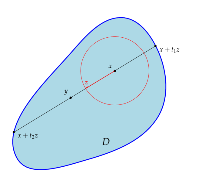
Perform a random walk Xn on a bounded convex domain D with boundary D: given Xn=x in D we choose a random one dimensional subspace [Z] and compute the length L of the segment of the line tx+tZ lying in D. This line intersects the boundary D in exactly two points x+t1Z, t1=t1(x,Z)<0 and x+t2Z, t2=t2(x,Z)>0, which terminate the segment. Finally we choose a 'random' point Xn+1=y on the segment and consider L as a function of x and y, i.e. L=L(x,y). This gives a Markov chain Xn. The Markov operator is given by Pf(x)=2vol(Sd1)Df(y)xyd1L(x,y)dy and since (x,y)xyd+1L(x,y)1 is symmetric Lebesgue measure on D is reversible.
We first have to clearify what is meant by a random one dimensional subspace. How do we choose such a subspace: We start with a random unit vector Z on Sd1, i.e the distribution of Z is the normalized surface measure on Sd1. Then we take the uniform distribution on the segment [x+t1Z,x+t2Z] of length L and choose a point on this segment randomly.
markov chain
This will give us the Markov operator Pf(x)=Sd1t1t2f(x+tz)L(x,x+tz)dtσ(dz)=Sd1(0t2f(x+tz)+0t1f(xtz))1L(x,x+tz)dtσ(dz)=Sd1(0t2(x,z)f(x+tz)L(x,x+tz)+0t2(x,z)f(xtz)L(x,xtz))dtσ(dz)=2Sd1(0t2(x,z)f(x+tz)L(x,x+tz)dtσ(dz)=2vol(Sd1)Df(y)L(x,y)xyd1dy . Here we used two simple facts: 1. for all t[t1,t2]: L(x,x+tz)=L(x,y), hence it doesn't depend on t, 2. t2(x,z)=t1(x,z) and finally integration in 'polar coordinates': if xD and t2 is the (euclidean) distance of x to the intersection point of the half line originating in x and pointing in direction z and the boundary of D, then Dg(y)dy=vol(Sd1)Sd10t2g(x+tz)td1dtσ(dz) applied to g(y)=f(y)xyd+1L(x,y)1.
Suppose 0 is an interior point of the convex domain DRd. Show that vol(D)vol(B2d)=Sd1pD(z)dσ(dz) . where B2d denotes the euclidean unit ball and pD(z):=inf{r>0:zrD} is the so called Minkowski functional of D, i.e. D=D=[pD<1] and D=[pD=1]. Suggested solution.
Write a subroutine which determines the numbers t1 and t2 given the Minkowski functional of D and two points x,yD.
Of course we may take any open and bounded set D with sufficiently 'nice' boundary. The problem is not the Markov operator - this doesn't change anyway - the problem is a possibly huge number of intersection points!
Suppose w1,,wn:SS are continuous maps on the Polish space S and p1,,pn:S[0,1] are continuous such that for all xS: pj(x)=1. Then Pf(x):=jpj(x)f(wj(x)) is a Markov operator on Cb(S). The corresponding Markov chain Xn is called a random iterated function system (IFS for short): we have P(Xn+1=wj(x)|Xn=x)=pj(x). If P:C0(S)C0(S) is Feller then the adjoint P:M(S)M(S) is given by Pμ(A)=jwjApjdμ and if all pj are constant: Pμ=pjμwj.
Given a stochastic matrix p(x,y) on a finite or countable set S with invariant probability measure μ. Verify that the adjoint of the Markov operator P:L2(μ)L2(μ) is given by Pf(x)=yf(y)q(x,y),whereq(x,y)=p(y,x)μ(y)μ(x) and conclude that μ is reversible iff x,yS:μ(x)p(x,y)=μ(y)p(y,x) . Give an example of a stochastic matrix with multiple reversible strictly positive measures. Suggested solution.
Suppose μ and ν. respectively, are reversible measures for the stochastic matrices P and Q, respectively. Then μν is a reversible measures for the Kronecker product PQ. If in addition both P and Q are ergodic, then PQ need not be ergodic (cf. exam).
Suppose S is finite and P:L2(μ)L2(μ) is a self-adjoint Markov operator, i.e. Pf(x)=p(x,y)f(y), yp(x,y)=1, p(x,y)0 and μ(x)p(x,y)=μ(y)p(y,x). Then for all fL2(μ): (1P)f,f=12x,yp(x,y)(f(x)f(y))2μ(x) 2. If for all x: μ(x)>0 and for xy: p(x,y)>0, then P is ergodic.
Put a(x,y)=p(x,y)δx(y), then ya(x,y)=0 and since μ is reversible: μ(x)a(x,y)=μ(y)a(y,x). Thus we get x,ya(x,y)f(x)2μ(x)=0andx,ya(x,y)f(y)2μ(x)=x,ya(y,x)f(y)2μ(y)=0 . Therefore (1P)f,f=x,ya(x,y)f(y)f(x)μ(x)=x,ya(x,y)(f(y)f(x)+12f(x)2+12f(y)2)μ(x)=12x,ya(x,y)(f(x)f(y))2μ(x)=12x,yp(x,y)(f(x)f(y))2μ(x) . 2. Suppose f(x1)f(x2), then (1P)f,f(f(x1)f(x2))2p(x1,x2)μ(x1)>0 .
S=ZN, p(x,x+1)=q(x+1), p(x,x)=r(x) and p(x,x1)=p(x1). In this case we have Pf(x)=p(x1)f(x1)+r(x)f(x)+q(x+1)f(x+1). A measure μ is reversible iff xq(x)p(x)=1andxZN:μ(x)=cy=0x1q(y+1)p(y),
S=Z, U:SR0+, p(x)=q(x)=eU(x)/2 and Z:=yZeU(y). A reversible probability measure is given by μ(x)=eU(x)/Z
We have a collection of N molecules in two boxes. Choose one of these molecules randomly and put it into the other box. We say that the system is in state xS:={0,,N} if there are exactly x molecules in the first box. For x<N we have: p(x,x+1)=(Nx)/N and for x>0: p(x,x1)=x/N, otherwise p(x,y)=0. Verify that the binomial distribution μ(x)=(Nx)2N is reversible. The corresponding Markov chain is called Ehrenfest chain.
We have got two boxes A and B, each of which contains exactly N balls. n of these balls are black and 2Nn balls are white. We say that these collection of balls is in state x, x=0,,n if box A contains x black balls. Now we choose 'randomly' one ball from each box and put the ball from box A into box B and the ball from box B into box A. This gives us a Markov chain on S={0,,n} - That's called the Bernoulli-Laplace diffusion model. Check that we have the following transition function for x,yS: p(x,y)={(Nx)(nx)N2if y=x+1 and ynx(nx)+(Nx)(N(nx))N2if y=xx(N(nx))N2if y=x1 and y00otherwise 2. Verify that the hypergeometric distribution μ(x)=(nx)(2Nnnx)/(2Nn) . is reversible.

Poissonization

Up until now we have been investigating a linear operator P and the semigroup Pn, nN0. Our next focus of interest is on so called one parameter semigroups Pt, which depend on a continuous parameter tR0+. There is an easy procedure to 'imbed' a discrete semigroup in a continuous semigroup: the Poissonization: Suppose E is a Banach space and P:EE a bounded linear operator; let Nt, t0, be a family of Poisson variables with parameter λ, i.e. P(Nt=n)=(λt)neλtn! then putting L:=P1 and Qt:=EPNt=n=0(λt)neλtn!Pn=eλtL we get a continuous contraction semigroup Qt, t0, with generator λL. Actually, for all xE the mapping tQtx is analytic. We remark that we do not have: Qn=Pn for nN, hence the quotation 'imbed'! Strict imbedding is not always possible.
If P is a bounded, strictly positive (definite) linear operator on a Hilbert space E (i.e. for some c>0 and all xE: Px,xcx2), then there is a bounded, positive (definite) linear operator L such that P=eL. 2. Find a symmetric stochastic matrix PM(2,R) for which there is no matrix LM(2,R) such that P=eL.
Qt is the family of Markov operators for a Markov process (Yt)t0, where the number of steps of the original Markov chain Xn (with Markov operator P) is Nt. i.e. Yt=XNt.
Suppose L=(ljk)M(n,R) has the following properties:
  1. For all j: kljk=0.
  2. For all jk: ljk0
Then the matrix etL is stochastic.
Proof: For sufficently large a>0 the entries of the matrix L+a are non-negative. Hence all entries of etL=et(L+a)at=et(La)eat are non-negative. Moreover, for x=(1,,1)t we get Lx=0 and thus: (pjk)x:=eLx=x, i.e. for all j: kpjk=1. qed
Let P be the Markov operator in exam. Put λ=1 and describe the Markov process with Markov operators Qt.
If P:B(S)B(S) has invariant measure μ, then for all t0 μ is invariant for Qt. 2. If P:L2(μ)L2(μ) is self-adjoint, then so is Qt:L2(μ)L2(μ) for all t0. 3. If Qt is ergodic then P:L2(μ)L2(μ) is ergodic.
If a finite stochastic matrix (p(x,y)), x,yS has the property that for each pair (x,y)S×S there is some nN0 such that p(n)(x,y)>0, then P has a unique invariant probability μ - hence it's ergodic with respect to μ. Here p(n)(x,y) are the matrix entries of the n-th power of the stochastic matrix. Hint: Use the remark following exam.
Verify that the Markov chains in exam, exam, exam and exam are ergodic.
For λ>0 let γn be an i.i.d. sequence of non-negative random variables with density λeλt. Put Γ0:=0 and Γn=j=1nγj. Then Γn has density λ(λt)n1(n1)!eλt . 2. Define Nt:=max{n0:Γnt}=inf{n1:Γn>t}1, then Nt is an increasing N0 valued process satisfying: [Ntn]=[Γn+1>t], [Ntn]=[Γnt] and nN0:P(Nt=n)=(λt)nn!eλt . Usually γ is interpreted as a waiting time for the arrival of a bus. In this case Γn is the waiting time for the arrival of the n-th bus and Nt is the number of buses that have arrived up to time t.

Pinsker- and Poincaré inequality

Proving ergodicity of a particular Markov operator might be quite intricate. One method of proof is based on Pinsker's inequality:
Suppose μ is a probability measure on S and f:SR0+ is such that fdμ=1. Then |f1|dμ2Ent(f) . This is called Pinsker's inequality. Hint: Use the elementary inequality: 3(x1)2(4+2x)(xlogxx+1), which holds for all x0. Suggested solution.
Now assume Pf=f, f0 and fdμ=1. If Ent(Pnf) converges to 0, then |f1|dμ=0, i.e. f is μ a.e. constant. Another related method is based on so called Poincaré inequalities: for all f such that fdμ=0 there is some constant CR+ such that f21Cf(1P)fdμ . This inequality immediately implies that if Pf=f then f is μ a.e. constant, i.e. f=fdμ. The constant C is called the spectral gap of the operator 1P, because in case 1P is self-adjoint, it's the distance of 0 to the rest of the spectrum of 1P - which is a subset of R+. The following generalizes exam:
Let Pf(x)=f(y)P(x,dy) be the Markov operator of a reversible Markov chain with reversible probability measure μ. Verify that for all fL2(μ): Q(f):=f(1P)fdμ=12(f(x)f(y))2P(x,dy)μ(dx) . If for all μ(A)>0 and μ almost all x: P(x,A)>0, then P is ergodic on L2(μ). Q is called the Dirichlet-form of P. 2. Verify that the functional fQ(f) is convex, i.e. Q((1t)f+tg)(1t)Q(f)+tQ(g).
Let Q be the Dirichlet-form of a self-adjoint Markov operator with reversible probability measure μ. Prove that Q(|f|)Q(f), Q(f+)Q(f) and for all sR: Q(fs)=Q(f). Conclude that Q(f)supsQ((fs)+).

Continuous Dynamical Systems

The spaces Cb(Rd), C0(Rd) and Cc(Rd) are called the space of all bounded and continuous functions, the space of all continuous functions vanishing at infinity and the space of all continuous functions with compact support. The first two spaces are Banach spaces with the norm given by: f:=sup{|f(x)|:xRd} . and Cc(Rd) is a dense subspace of C0(Rd). By C(Rd) and Cc(Rd) we denote the space of all smooth functions and the space of all smooth functions with compact support. Both are dense subspaces of C0(Rd).
Suppose ζ:RdRd is smooth, then by the existence theorem of ordinary differential equations there is an open subset D of R×Rd such that {0}×RdD and a smooth mapping θ:DRd such that (CDS1)tθ(t,x)=ζ(θ(t,x))andθ(0,x)=x . By the uniqueness theorem of ordinary differential equations this map has the additional property that for all xRd and all t,s>0: θ(t+s,x)=θ(t,θ(s,x)), whenever θ(s,x) and θ(t,θ(s,x)) are defined. Putting Ptf(x):=f(θ(t,x)) we get a local group on C0(Rd) with the property that for all fC(Rd) and all (t,x)D: (CDS2)tPtf(x)=j=1dtθj(t,x)jf(θ(t,x))=j=1dζj(θ(t,x))jPtf(x) . For a manifold M the spaces C0(M), C(M) and Cc(M) are defined analogously.

Vector fields

A vector field X on a manifold M is a linear mapping X:C(M)C(M) such that for all f,gC(M): X(fg)=fXg+gXf
Of course, the space Γ(M) of all vector fields on M is a vector-space ((X+Y)f:=Xf+Yf), but it's also an C(M)-modul: for all gC(M) and all vector fields X there is a new vector field gX: (gX)f(x):=g(x)Xf(x). Moreover, given two vector fields X and Y the commutator [X,Y]:=XYYX is also a vector field.
Prove that the commutator is indeed a vector field.
Straightforward insertion shows that the commutator satisfies Jacobi's identity: [X,[Y,Z]]+[X,[Y,Z]]+[X,[Y,Z]]=0 and [X,Y]=[Y,X]. Thus Γ(M) is a Lie-algebra (cf. e.g. wikipedia).
Prove that the vector space R3 with the vector product (x,y)x×y is a Lie-algebra, i.e. x×y=y×x and x×(y×z)+y×(z×x)+z×(x×y)=0.
Vector fields and smooth mappings ζ:MRd on open subsets M of Rd are in one to one correspondence: for any such mapping ζ (CDS3)Xf(x):=j=1dζj(x)jf(x) is a vector field. The mapping θ:DRd defined in (CDS1) is called the flow of the vector field X and the curve c(t):=θ(t,x) is called the integral curve of X through x. Instead of Xf(x) we will also write Xxf. Conversely, for a vector field X on M there is exactly one smooth mapping ζ:MRd, such that (CDS3) holds - this is usually one of the first results in any course on manifolds. If a smooth mapping θ:DM satisfies (CDS1), then: (CDS4)fC(M):t(fθ)(t,x)=Xf(θ(t,x))=PtXf(x) . On the other hand this relation implies (CDS1): just take for f the projections (x1,,xd)xj onto the components. In case M is an arbitrary manifold we take (CDS4) just as definition of the flow θ of a vector field X.
A constant vector field E=ejj on Rd commutes with any other constant vector field and the flow of E ist given by σ(t,x)=x+te.
If D(X):=D=R×M, the vector field X is said to be complete. Completeness of X ensures that Ptf(x):=f(θ(t,x)) is in fact a group on C(M), Cb(M), C0(M), etc.; moreover, the mappings θt:MM are diffeomorphisms for all tR with inverse θt.
The vector field Xx=x2x on R is not complete.
Find a solution of the first order PDE tu=yxuxy on M=R2 satisfying u(0,x,y)=x2y2. Suggested solution.

From vector fields to one parameter groups

Putting t=0 in (CDS4) we see that the group Pt, tR, also determines X: Xf(x)=t|t=0Ptf(x)=limt01t(Ptf(x)f(x)) . The notion of a complete vector field allows us to write (CDS1) as (CDS4). By the group property we get: XPtf(x)=lims01s(Pt+sf(x)Ptf(x))=lims01s(Psf(θt(x)))Ptf(θt(x)))=Xf(θt(x))=PtXf(x)i.e.PtX=XPt and thus (CDS1) is equivalent to: (CDS5)tRfC(M):tPtf(x)=XPtf(x) .
Suppose X is a vector field on M and u:MR+ is smooth such that
  1. For all r>0 the set [ur] is compact.
  2. There exists a constant C>0, such that XuCu.
Then X is complete.
Proof: For any xM put c(t):=θ(t,x). Then it follows by 2. and (CDS5) that ddt(eCtu(c(t)))=eCt(Xu(c(t))Cu(t))0, i.e: u(c(t))u(x)eCt, which shows that c(t) is in the compact set [uu(x)eCt]. qed
If ζ is L-Lipschitz on Rd, then X=ζjj is complete on Rd.
Proof: Choose u(x)=x2+1 then Xu=jζjju=2j(ζjζj(0))xj+2jζj(0)xj2Lx2+2KxCu(x) . qed
Next we are going to verify that Ptf=fθt it is a continuous group on C0(M) meaning that for all fC0(M) the map tPtf is a continuous curve in C0(M). Indeed, for fC0(M), there is some ϵ>0, some δ>0 and a compact subset K of M, such that for all d(x,y)<δ: |f(x)f(y)|<ϵ and |f|Kc|<ϵ. Moreover, we can find some r>0, such that for all |t|<r, all xK: d(x,θt(x))<δ and |f|θt(Kc)|<ϵ. It follows that PtffsupxK|f(θt(x))f(x)|+supxKc|f(θt(x))|+supxKc|f(x)|ϵ+ϵ+ϵ . In general the group Pt is not continuous on Cb(M): take for example M=R, Ptf(x):=f(x+t) and f(x)=sin(x2); for all t>0: supx|sin((x+t)2)sinx2|=2. However for fCc(M) we conclude by the mean value theorem of calculus that: 1t(Ptff)Xfsup{|sf(θ(s,x))sf(θ(0,x))|:0<s<t,xM} . As f has compact support this converges to 0 as t converges to 0 and hence Xf is the derivative of the curve tPtf in C0(M) at t=0. In fact equation
(CDS5) is somewhat weaker than the linear ordinary differential equation in C0(M): (CDS6)ddtPtf=XPtf . Beware, on the left hand side we mean the derivative of a Banach space valued curve! What's the asset? (CDS6) is linear! The price for this 'linearization' of the non-linear differential equation x(t)=ζ(x(t)) is the substitution of the infinite dimensional space C0(M) for the finite dimensional space M. On the other hand we may and will examine (CDS6) in different Banach spaces such as Lp(μ) for some measure μ on M and in these cases the evaluation of (CDS6) at a particular point doesn't make sense in general, though it makes sense in e.g. C0(M). As a final remark we notice that for all fC(M), all xM and all nN we have: dndtn|t=0Ptf(x)=Xnf(x) Thus in case tPtf is analytic we get the Taylor expansion: Ptf=n=0tnn!Xnf which we simply write as etXf. Henceforth we will use etX just as a synonym for Pt. Take for example M=Rd, h=(h1,,hd)Rd and put X=hjj, then: θ(t,x)=x+th and etXf(x)=f(x+th). On the other hand we have in case tf(x+th) is analytic (which is obviously weaker than analyticity of tPtf): etXf(x)=n=0tnn!(hjj)nf(x) and thus we are back at the classical Taylor formula: f(x+th)=etXf(x).
Let θ be the flow of the complete vector field X and Ptf=fθt. A Borel measure μ on M is said to be invariant under θ if tRfCc(M):Ptfdμ=fdμ .
Of course this implies that Xfdμ=0. Conversely, since Pt maps Cc(M) into itself, we get for every fCc(M) by (CDS6): ddtPtfdμ=XPtfdμ=0 and thus μ is invariant iff for all fCc(M): Xfdμ=0.
Suppose X is a complete vector field on a Riemannian manifold M, ρC(M) the density of a Borel measure μ with respect to the Riemannian volume v. μ is invariant under the flow of X if and only if div(ρX)=0.
Proof: The divergence divY of a vector field Y on M may be defined by (CDS7)gCc(M):Ygdv=gdiv(Y)dv. . Now take any fCc(M), then Xfdμ=(ρX)fdv=div(ρX)fdv Since fCc(M) is arbitrary, the conclusion follows. qed
Verify that in the euclidean case (CDS7) amounts to div(ζjj)=jζj .
Provided the conditions of the above theorem are satisfied the group Ptf:=fθt will turn out to be a continuous group on both C0(M) and Lp(μ) (for all 1p<). As for ergodicity of the flow we have a negative result: If H:MR is a first integral of the vector field X, i.e. H is not constant and XH=0, then θt is not ergodic. First integrals are an important means in ODE, for they are obviously constant along integral curves, i.e. for all xM the function tH(θt(x)) is constant! Anyway, if Ptf:=fθt is ergodic, then there is no first integral.

Integrating factor

Let X=Q(x,y)x+P(x,y)y be a vector field on an open subset M of R2, then div(ρX)=x(ρQ)+y(ρP) and thus div(ρX)=0 if and only if ρ is an integrating factor of the differential equation: c1(t)=Q(c1(t),c2(t))andc2(t)=P(c1(t),c2(t)) i.e. c(t)=(c1(t),c2(t)) is an integral curve of X. If ρ is an integrating factor and M is simply connected, then there is a first integral H given by xH=ρQandyH=ρP .
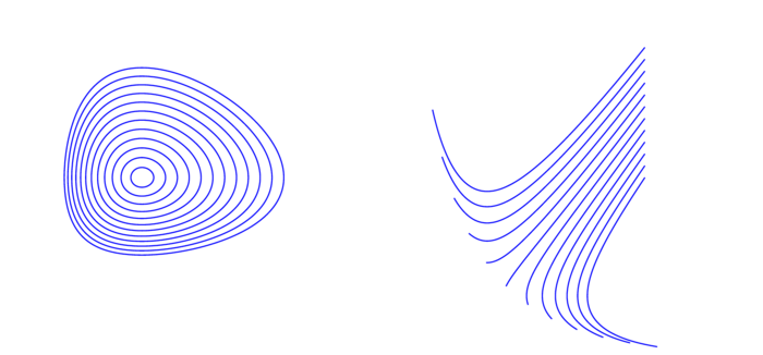
The predator-prey model is the flow of the vector field X=(axbxy)x+(cxydy)y on M=R+×R+ for a,b,c,d>0. Verify that the following measure is invariant: μ(K)=K1xydxdy . Here x and y model the 'densities' (the number of individuals per unit area) of the prey and the predators, respectively. 2. Verify that H(x,y)=cxbydlogx+alogy is a first integral and that H is strictly convex. If a,b>0 and c,d<0 this is called the competitor model.
Some trajectories for the predator-prey and the competitor model:
models

Geodesic flow

Let M be a Riemannian manifold and G the so called geodesic vector field, i.e. for all XmTmM the tangent vector GXmTXmTM is horizontal and π(XXm)=Xm. The flow G(t,Xm) of this field is the parallel transport of Xm along the geodesic texpm(tXm). Then the Riemannian volume on TTM is invarian under Gt. If M is an open subset of Rd we have TM=M×Rd and for the cannonical Riemannian metric on M we get G(x,v)=jvjxjand its flow:G(t,x,v)=(x+tv,v) Every measure of the form dμ(x,v)=ρ(v)dxdv is invariant under the flow G, indeed: div(ρG)=j(xj(ρ(v)vj)+vj0)=0 . A typical choice is ρ(v)=cexp(v2/2). If the geodesic flow is complete, the Riemannian manifold M is said to be complete
. Quite miraculously (cf. Hopf-Rinow Theorem) this happens if and only if the manifold M furnished with the geodesic metric (cf. e.g. (DIF4)) is a complete metric space.

Hamiltonian flow

Let (M,.,.) be a Riemannian manifold and π:TMM the canonical projection, i.e. for all mM and all XmTmM: π(Xm)=m. Suppose ω1 is the cannonical 1-form on TM, i.e. ω1(XXm)=π(XXm),Xm and H:TMR is a smooth function, a so called Hamiltonian. The Hamiltonian vector field XH on TM is defined by dH=XHdω1. Then the Riemannian volume on TM is invariant under the flow of the Hamiltonian vector field XH. On TRd=Rd×Rd this field is given by X(q,p)H:=j=1d(pjHqjqjHpj) . The flow of this vector field is a collection of curves t(q1(t),,qn(t),p1(t),,pn(t))=(q(t),p(t)) (the integral curves), which satisfy the so called Hamilton equations: qj(t)=pjH(q(t),p(t)),pj(t)=pjH(q(t),p(t)) simply written as qj=pjH and pj=qjH.
Verify that H is a first integral of the Hamiltonian flow.
Hence ergodicity of the Hamiltonian flow is usually investigated on submanifolds [H=const]; the density of an invariant measure on this manifold with respect to the Riemannian measure on [H=const] is given by 1/H.
Determine the Hamilton equations for H(q,p)=12mpj2+U(q) for some smooth function U:M(Rd)R. Check that these are the Newtonian equations of a particle of mass m moving in a potential U. 2. Verify for m=1, E,α>0 and U(q)=qα/α that the set [H=E] is a compact submanifold of Rd×Rd and compute H for (q,p)[H=E].
The motion of a particle of mass m and charge q in a stationary electromagnetic field is described by the Lorentz equation: mddtv=q(E+v×B),ddtx=v, where E and B are vector fields on M=R3 (they are called the electric and the magnetic field respectively). Put X:=j=13vjxj+qj=13(Ej+(v×B)j)vj, then the Lebesgue measure on R6 is invariant under the flow of X.

Diffusions

In what is going to follow we construct a model describing the distribution of temperature in an infinite rod: The basic assumptions are as follows:
  1. There is no heat transfer into its environment.
  2. The change of temperature in time at any point is proportional to the differences in temperature to its neighbours.
Fix some numbers Δx,Δt>0 and take for nZ: x{nΔx:nZ} and t{nΔt:nN}. We assume the rod is made of a series of molecules in fixed positions x. By u(x,t) we denote the temperature (i.e. the kinetic energy) at times t of the molecule in position x. This molecule has two relevant neighbours located in positions xΔx and x+Δx, respectively. The second assumption implies that u(x,t+Δt)u(x,t)=a(x)((u(xΔx,t)u(x,t))+(u(x+Δx,t)u(x,t))) . The condition a(x)>0 says that the temperature in x can only increase if u(x,t)<12((u(xΔx,t)+(u(x+Δx,t)), meaning that the temperature in x is smaller than the mean temperature of its neighbours. In the continuous case (i.e. xR, tR+) there is only one reasonable analogon: tu(x,t)=a(x)x2u(x,t) If a(x)>0 this equation is called a diffusion equation. The general form of which is given by tu(x,t)=a(x)x2u(x,t)+b(x,t)xu(x,t) . The factor b is called the drift of the diffusion. For a=1 and b=0 this is known as the heat equation on the real line.

A probabilistic interpretation

We construct very simple Markov chains approximating a Markov process known as Brownian motion: For x{nΔx:nZ} let us call the interval (xΔx/2,x+Δx/2) the box about x. A particle moving on the real line R obeys the following rules:
  1. At time t=0 the particle is located in the box about y.
  2. If at time t=0,Δt,2Δt, the particle is located in the box about x the probability of finding the particle at time t+Δt in the boxes about xΔx and x+Δx is 1/2.
Let us denote by p(x,t)Δx the probability of finding the particle at time t in the box about x. By assumption the probability of finding the particle at time t+Δt in the box about x is given by p(x,t+Δt)Δx=12p(xΔx,t)Δx+12p(x+Δx,t)Δx, this is because with probability 1/2 the particle has moved from the box about xΔx or from the box about xΔx to the box about x. Thus we obtain p(x,t+Δt)p(x,t)=12(p(xΔx,t)p(x,t)+p(x+Δx,t)p(x,t))=12(p(xΔx,t)2p(x,t)+p(x+Δx,t)) . Putting Δx=Δt and letting Δt0 we get (DIF1)tp(x,t)=12x2p(x,t) . For any yR the function py(x,t):=12πtexp(12t(xy)2) solves the PDE
(DIF1); moreover it has the following properties py(x,t)0,Rpy(x,t)dx=1andr>0: limt0yry+rpy(x,t)dx=1 . The first two properties express the fact that xpy(x,t) is the density of a probability measure: the probability of finding the particle at time t in the interval (α,β) is given by αβpy(x,t)dx. The third property reflects the initial condition: at time t=0 the particle is located in position y, i.e. the probability of finding the particle in any interval of the form (yr,y+r) at about y equals 1.

Heat semigroup on Rd

Let Δ:=j2 be the Laplace operator on Rd. The heat equation on Rd is tu=Δu:=j2u . For any fC0(Rd) there is a unique bounded solution u(t,x) satisfying u(0,x)=f(x): Ptf(x):=u(t,x)=f(xy)pt(y)dy=f(y)pt(xy)dy=fpt(x) . Here pt(y) denotes the heat kernel of Rd: pt(y):=(4πt)d/2ey2/4t . The family of operators Pt forms a so called continuous contraction semigroup on the space C0(Rd) with generator Δ, i.e. fCc(Rd):limt0Ptfft=Δf and the limit is in C0(Rd). Moreover, it's also a continuous contraction semigroup on the spaces Lp(Rd) for 1p<: for fLp(Rd), gLq(Rd), 1/p+1/q=1, we conclude by Hölder's inequality: |Ptf(x)g(x)dx||f(xy)g(x)pt(y)|dxdyfpgq i.e. Pt:Lp(Rd)Lp(Rd)1. Usually it's not that difficult to verify continuity of these semigroups (cf. lemma). However the following provides an altenative way for p=2:
The Fourier transform of the heat kernel pt is given by p^t(y):=cdpt(x)eix,ydx=cdety2wherecd=(2π)d/2 .
  1. Conclude from this fact that pspt=ps+t, i.e. Pt is a semigroup.
  2. For all fL2(Rd) the map fPtf is continuous.
  3. For all fH2(Rd): Ptfft+Δf212tfH2,wherefHs2:=|f^(y)|2(1+y2)sdy . Thus Δ is the generator of the heat semigroup on L2(Rd) and dom(Δ)H2(Rd).
1. The formula can be checked by straightforward calculation. However another way to derive the formula for the Fourier transform of Pt is as follows: the Fourier transform of Δf is yy2f^(y) and thus the Fourier transform of etΔf is yety2f^(y). Now, since cdp^s+t=p^s.p^t it follows that pspt=ps+t and thus Pt is a semigroup.
2. We simply utilize the fact that ff^ is an isometry on L2(Rd) and it maps the Laplacian to multiplication by .2! The Fourier transform of Ptf is yety2f^(y) and thus: fPtf22=|1ety2|2|f^(y)|2dy and by dominated convergence this converges to 0 as t converges to 0. 3. Similarly Ptfft+Δf22=t2(ety21+ty2t2(1+y2))2(1+y2)2f^(y)dyt2supr>0|er1+rr2|fH22=12t2fH22 .
For f,gL1(Rd) and gL1(Rd) we have: |Ptf(x)g(x)dx|f1g1pt and thus: Pt:L1(Rd)L(Rd)(4πt)d/2 - Pt is said to be ultracontractive. Solution by T. Speckhofer.
Suppose fL2(Rd) satisfies Ptf=f for some t>0. Prove that f=0. Hint: Use the Fourier transform.

The heat semigroup on Td

As the heat semigroup on Rd doesn't admit an invariant probability measures we give another example based on the heat semigroup on Rd, which has an invariant probability measure. The heat semigroup on Td is exactly of the sort of examples we have in mind when talking about ergodic semigroups!
Verify that the heat kernel of the d-dimensional torus Td is given by t>0 xTd:qt(x):=nZdpt(x+2πn) . Just check that qt is the density of a probability measure on Td and tqt(x)=Δqt(x).
The associated semigroup on L2(Td) is self-adjoint and ergodic, i.e. if Ptf=f for all t>0, then f ist constant. Indeed, the semigroup Pt on L2(Td) is Ptf(x)=Tdqt(y)f(xy)dy=Tdqt(xy)f(y)dy which is self-adjoint for (x,y)qt(xy) is symmetric. For fC(Td) let FCb(Rd) denote the periodic extension of f, then Ptf(x)=TdnZdpt(xy2πn)f(y)dy=Rdpt(xy)F(y)dy . Thus the heat semigroup on Td applied to fC(Td) is just the heat semigroup on Rd applied to the periodic extension F of f. Now em(x):=eix,m, mZd, is an orthonormal basis for the Hilbert space L2(Td); by the preceeding formula and exam we get: Ptem(x)=Rdpt(y)eixy,mdy=etm2eix,m . Assume Ptf=f for f=cmemL2(Td) then: cmem=cmetm2em, which can only hold if for all m0: cm=0, i.e. f is constant: The heat semigroup on L2(Td) is ergodic!
For fL2(Rd) and xTd put F(x):=nZdf(x+2πn), Then the Fourier transform of F in Td at mZd concides with the Fourier transform of f in Rd at mZd up to a constant factor: F^(m)=cdf^(m).
Prove that the Fourier transform of qt (on Td) is q^t(n)=etn2 (nZd) and verify that for all fL2(Td): Ptf^(n)=etn2f^(n).

Diffusion semigroups

Let (M,.,.) be a Riemannian manifold with Riemannian metric .,. and Riemannian volume v. Suppose a,ρ:MR+ are strictly positive and smooth - actually by adjusting the Riemannian metric we way assume that a=1 (cf.
subsection) . Put μ(dx)=ρ(x)v(dx) and let X be a vector field such that (aρ)+ρX=0 - in this case the measure μ is called the speed measure of H. The operator Hf=aΔf+XfwhereΔf:=div(f), is a densly defined, symmetric and positive (definite) operator on L2(μ), i.e. Hf is defined for all f in the dense subspace Cc(M) of L2(μ) and f,gCc(M):Mf.Hgdμ=MHf.gdμandMf.Hfdμ0 . All of this follows from
Under the above conditions for a,ρ and X we have for all f,gCc(M) the following relation (DIF2)MHf.gdμ=Mag,fdμ .
Proof: By definition of the divergence (cf. theorem) we have: agρΔfdv=(agρ),fdv and by assumption we infer that: Hf.gdμ=agρΔf+gρXfdv=(agρ),f+gρXfdv=(aρ),fg+g,faρ+gρX,fdv=g,fadμ . qed
If a=1 and X=U, then ρ=eU. In the particular case M=Rd, U(x)=x2/2 we get the diffusion operator Hf(x)=j2f(x)+xjjf(x) . Its speed measure is the standard gaussian measure γ on Rd, i.e. the density of γ is given by (2π)d/2ex2/2 .
If a,ρ and X satisfy the conditions of lemma and if μ is a probability measure, then the operator H (or H) is called a diffusion operator on M and it generates a diffusion semigroup Pt=etH. Actually any densly defined, positive, symmetric operator H0 on a Hilbert space E generates a continuous contraction semigroup Pt. This is because any such operator can be extended to a self-adjoint (unbounded) linear operator H (the so called Friedrichs extension). The semigroup Pt:=etH is a continuous contraction semigroup with generator H - this is more or less a special case of the Hille-Yosida Theorem (cf. theorem). If H is a diffusion operator, then the relation (DIF2) also holds for f=g in the domain of the extension! In finite dimensions all of this is pretty obvious, nonetheless worth mentioning because it already comprises all the essential results (cf. e.g. theorem):
If H is a positive, self-adjoint operator on a finite dimensional Hilbert space (i.e. a euclidean space), then Pt:=etH is a self-adjoint, continuous contraction semigroup. If H is a self-adjoint operator on a finite dimensional Hilbert space, then Ut:=eitH is a continuous group of isometries. 2. Prove that (suggested solution) limT1T0TPtxdt=limT1T0TUtxdt=PrkerHx is the orthogonal projection onto the kernel of H (compare exam). This easily extends to the infinite dimensional case provided we have a spectral decomposition of H:dom(H)(E)E of the form (cf. exam): Hx=j=1λjx,xjxj,dom(H):={xE:λj2x,xj2<},λj0 .
That's the case for a diffusion on a compact Riemannian manifold. In general the diffusion semigroup Pt generated by H sends any fL1(μ) onto a smooth function. If the Riemannian manifold is complete and satisfies a certain geometric condition then Pt is Feller. The associated Markov process Bt, t0, is reversible with respect to the speed measure μ - in case a=12 the Markov process Bt is called Brownian motion on M with drift X.
If H is a diffusion operator on a complete Riemannian manifold with Ricci curvature bounded from below, then the associated diffusion semigroup is ergodic.
Proof: Once we know that the corresponding diffusion semigroup Pt, t>0, maps any fL1(μ) onto a smooth function, a solution of Ptf=f must be smooth and thus Hf=0. By lemma - and its extension to functions in the domain of H - we infer that 0=f.Hfdμ=af2dμ and since a,ρ are strictly positive: f=0 and thus f must be constant. qed
This in particular applies to compact Riemannian manifolds, to all complete manifolds of constant curvature, e.g. Rd or the hyperbolic spaces Hd.
Suppose M is an open interval, possibly unbounded, a,ρ:MR+ strictly positive and smooth, b:MR smooth and μ(dx)=ρ(x)dx such that (aρ)+ρb=0, i.e. for some x0M and cR+: ρ(x)=cexp(x0xa(y)+b(y)a(y)dy) Then Hu:=au+bu is a densly defined positive (definite) symmetric operator on L2(μ).
In any case ergodicity of the following examples can be checked directly; as in exam you just need to know all eigen functions of the diffusion operator:
The following are classical diffusion operators on open intervals. Prove that all of them generate ergodic semigroups (cf. e.g. exam). Suggested solution.
  1. M=(1,1), a(x)=1x2, b(x)=2x for some α,β>1. Compute the density ρ. The Jacobi polynomials Pn(α,β) are eigen functions of H for the eigenvalues λn=n(n+α+β+1) and they form a complete orthogonal set. For α=β these polynomials are called ultraspherical or Gegenbauer polynomials.
  2. M=R, a(x)=1, b(x)=2x. Compute the density ρ. The Hermite polynomials Hn are eigen functions of H for the eigenvalues λn=2n and they form a complete orthogonal set.
  3. M=R+, a(x)=x, b(x)=xα1 for some α>1. Compute the density ρ. The Laguerre polynomials Lnα are eigen functions of H for the eigenvalues λn=n and they form a complete orthogonal set.

Adjusting geometry

On e.g. a domain M of Rd a diffusion operator H is commonly defined as a second order partial differential operator: (DIF3)Hf:=j,kajkjkf+bjj where ajk, bj are smooth functions such that A(x):=(ajk(x)) is symmetric and strictly positive definite. However any diffusion operator on a domain can be written as the sum of the Laplacian and a vector field, we just need to define a suitable Riemannian metric:
Put (gjk):=A1, then we get for the Laplace operator on the Riemannian manifold M:=(M,(gjk)): Δf=j,kajkjkf+Xf , where the vector field is given by X=jζj(x)j with ζj:=kk(ajkG)GandG:=det(gjk)=1detA .
The Riemannian metric (gjk) induces the geodesic distance: (DIF4)dg(x,y):=inf{L(c):c:[0,1]M smooth, c(0)=x,c(1)=y} where L(c):=01gjk(c(t))cj(t)ck(t)dt is called the length of the curve c in (M,(gjk)). This is particularly easy to compute in case the dimension equals 1, for there is only one curve connecting two points (modulo reparametrization): c(t)=x+t(yx).
The interval M:=R+ with the Riemannian metric g(x)=1/x produces the geodesic distance x,yM:dg(x,y)=01|c(t)|c(t)dt=2|yx| (M,dg) is not complete!.
The interval M:=(1,1) with the Riemannian metric g(x)=1/(1x2) produces the geodesic distance dg(x,y)=2|arcsinyarcsinx|. Check that (M,dg) is not complete!
Thus neither the first nor the last example in exam is covered by proposition!
The interval M:=R+ with the Riemannian metric g(x)=1/x2 produces the geodesic distance dg(x,y)=|log(x/y)|. Verify that (M,dg) is complete.
Find a Riemannian metric on M:=(1,1) such that (M,dg) is complete.
Consider the diffusion operator (DIF3) on a bounded domain M in Rd with smooth boundary under Neumann boundary conditions (i.e. for all xM: f(x),N(x)=0). 1. If for some smooth function U - here a smooth function will always be defined in a neighborhood of M: j:kajkkU=bj+kkajk . Then ρ:=eU is the smooth density of a speed measure μ, i.e. for all smooth f,g satisfying the boundary conditions: Mf(x)Hg(x)μ(dx)=Majk(x)jf(x)kg(x)μ(dx) . 2. Conclude that if μ is a probability measure then any smooth function f satisfying both the boundary conditions and Hf=0 must be constant. 3. Altenatively, use Zaremba's principle (or Hopf's lemma) to prove 2. - this way you see that the speed measure doesn't matter at all!

Convolution semigroups

We just talk about convolution semigroups on R+: suppose μt, t>0, is a family of probability measures on R+ such that for all s,t>0: μsμt=μs+t, where μsμt((0,x]):=(0,x]μs((0,xy])μt(dy) is the convolution of μs and μt. The 1/2-stable distribution defined in exam is a prominent example. Here are a few more:
For t>0 let μt be the measure on R+ with density xexxt1Γ(t) . Show that the Laplace transform of μt is given by ωt(y)=(1+y)t. 2. Conclude that μsμt=μs+t. The measure μt is called the Γ-distribution with parameter t. 3. Compute xμt(dx). Suggested solution.
For t>0 let μt be the measure on N0 with density ntnetn! . Show that the Laplace transform of μt is given by ωt(y)=exp(ty(1ey)). 2. Conclude that μsμt=μs+t. The measure μt is called the Poisson distribution with parameter t. 3. Compute xμt(dx).
Suppose μt, t>0, is a family of probability measures on R+. Assume that its Laplace transform φt is given by φt(y)=exp(t01exyxν(dx)) For 0<p<1 let ν be the measure on R+ with density xpΓ(1p)xp . Show that for all y>0: 01exyxν(dx)=yp .
All these are particular cases of so called infinitely divisible distributions, cf. e.g. wikipedia.
← Introduction → Continuous Contraction Semigroups

<Home>
Last modified: Mon Aug 26 13:00:51 CEST 2024